Generating Diverse Training Environments for Autonomous Cyber Defense

Problem and motivation

#

Threat modeling is a field within cybersecurity generally aimed at identifying potential attack paths through some system of interest and evaluating the effectiveness of defensive strategies. A common representation of attack scenarios is the attack graph, in which nodes represent possible attacker actions and edges represent causal dependencies between those actions. The graph below shows a very minimal example of this.

graph LR;

A(Expose the
target service);

B(Send crafted
request);

C(Gain
unauthorized
access);

D(Read sensitive
data);

A-->B-->C-->D;

Due to the scale and complexity of modern infrastructure it is relatively rare to manually construct attack graphs for realistic systems. Instead, you typically create an explicit model of the system itself (its assets/components and the associations/relations between those assets), from which an attack graph can be automatically generated/derived.

One framework that facilitates the automatic generation of an attack graph from a model of a system is the Meta Attack Language (MAL). Simply put, MAL allows you to define asset types and association types, along with the attack actions that can be taken against each asset and how one successful attack may enable the next one. You model your system using the defined asset and association types, and the corresponding attack graph is implicitly embedded within the model.

As an illustrative example we can consider trainingLang — a small such MAL language — which defines the asset types Host, Network, User and Data. A minimal system could consist of a single host on a network, with one user and some data. This system model can be represented as a graph, as shown to the left in the figure below.

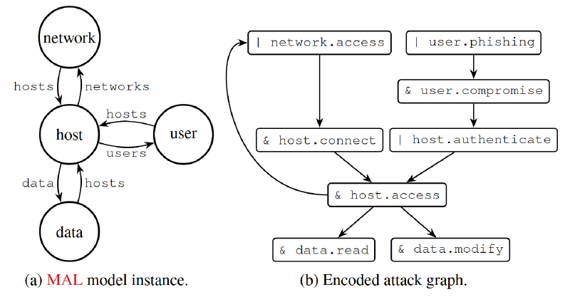
To the right in the figure we see the attack graph that the system model encodes, which MAL-tooling derives automatically without any additional effort from the modeler. &-nodes require all prerequisite attack steps to be completed, while |-nodes require only one prerequisite.

With the rise of AI, much of threat modeling research has begun to pivot towards training autonomous cyber defence agents based on machine learning and statistical learning approaches. The agents learn defensive policies by interacting with simulated attack scenarios; simulations often run on the kinds of attack graphs that we’ve just discussed.

While an AI trained on an attack graph could learn to defend the corresponding system very well, one has to consider the problem of overfitting. If we reconfigure our real-life system even slightly it no longer corresponds to that of which the AI agent learnt to defend. Consequently, the agent will likely perform much more poorly than in the original configuration. This is especially concerning since real-life systems can be reconfigured considerably more frequently than the time it may take to train these defenders.

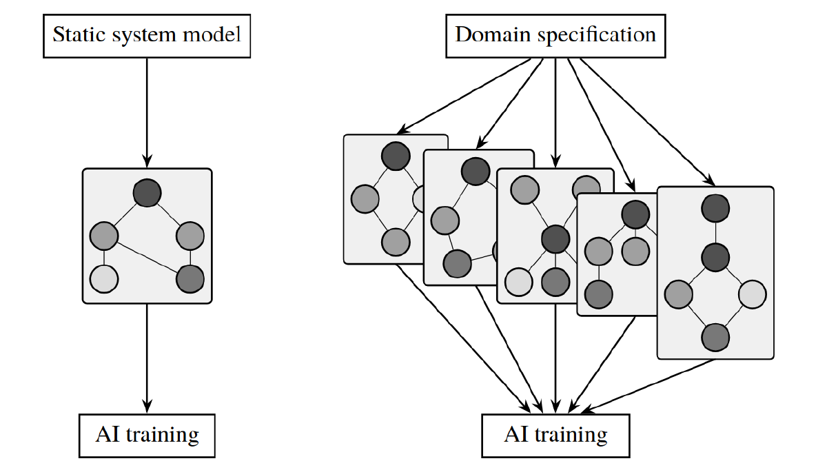
A better approach is to instead train the AI to defend not a single specific system, but a family (a domain) of systems. This family would ideally capture common architectural and security patterns while containing controlled variation across multiple dimensions. For example, instead of training the AI on a network with a fixed number of hosts and users, we train it on multiple attack graphs, each with a different number of hosts and users.

As of now, a researcher/modeller would have to manually (or programmatically) build each system model for the wanted domain. What is missing is a way to describe systems at a level of abstraction above individual system models. With such a solution the modeller would simply write a single domain specification from which any number of diverse and valid system models can be sampled and automatically generated.

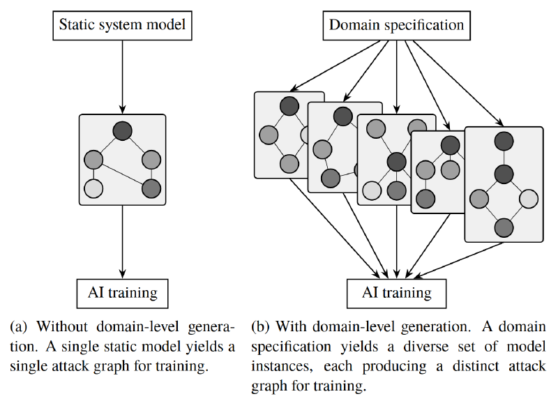
This — a domain-level model generation framework — is exactly what I set out to create.

A solution

#

Before detailing my proposed solution (InstaMAL), I’ll first cover the random wiring primitive that serves as its foundation.

Note that the system models we want to describe and generate can be represented as graphs. The problem is really to describe and generate random graphs that are valid system models. The graphs we are working with are heterogeneous in the sense that nodes and edges are typed, and directed in the sense that the direction of the edges carry meaning.

A new geometric random wiring primitive for heterogeneous graphs

#

Most random graph primitives are formulated for undirected non-typed graphs and cannot be directly used for our purposes.

The closest related work I could find, the random network generation procedure of Microsoft’s CyberBattleSim, uses a heterogeneous generalization of the stochastic block model (SBM). The SBM allows for controlled variability, but it can be quite difficult to tune all the parameters to your liking. In CyberBattleSim the parameters are simply hard coded, but for our purposes we want to leave all the control to the modeller.

A random graph primitive that has fewer parameters and that I found to be more intuitive is the random geometric graph (RGG). It works as follows:

“Scatter \(n\) nodes randomly in the unit square and connect any two nodes whose distance to each other is less than \(r\).”

The only parameters needed are the number of nodes \(n\) and the distance threshold \(r\). The geometric nature of the RGG makes it easier to grasp than, say, the SBM. A larger \(r\) makes it more likely that any two nodes fall within that distance of each other, making the graphs more connected. As \(r\) approaches \(\sqrt{2}\) (the length of the diagonal of the square) the graphs approach complete graphs. The figure bellow illustrates this, with the same 20 node positions but varying values of \(r\).

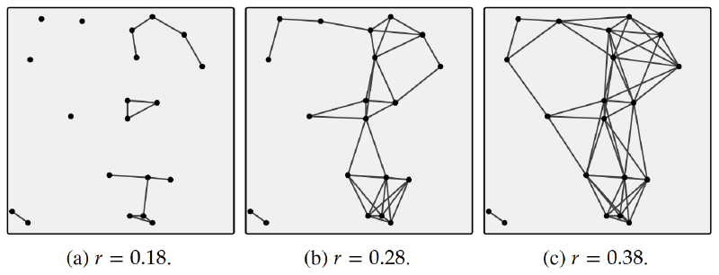
Furthermore, increasing \(n\) makes the unit square “more crowded”, also producing more connected graphs.

To fit our purposes we have to generalize the RGG to a directed heterogeneous version. The directed heterogeneous RGG (DHRGG) takes as input a set of typed nodes (replacing \(n\)) and a list of connection rules (replacing \(r\)). Each connection rule specifies a source node type, destination node type, edge type, as well as its own threshold radius. The specified nodes are scattered randomly in the unit square. Then, for each connection rule, a directed edge of the specified type is added between any eligible source-destination pair whose distance to each other falls within the rule’s radius.

The figure below shows an example of the classical RGG next to a corresponding DHRGG with two connection rules.

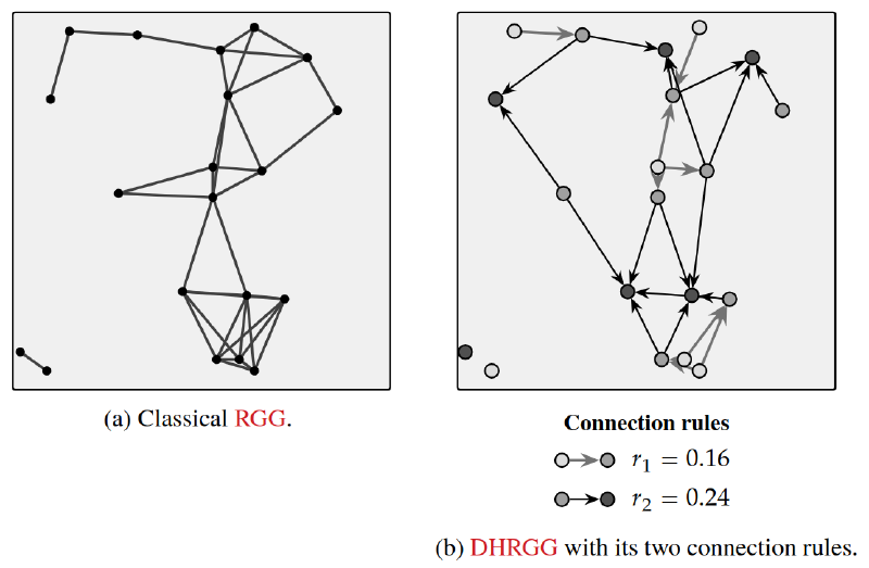
Now, I want to take a moment to think about how the DHRGG could help us to solve our problem. We can supply the DHRGG with, say, 2 Network nodes, 10 Host nodes and 10-20 User nodes to be randomly distributed in the unit square. In that case we can supply three connection rules: one that connects each network to all other networks (set source and destination types to Network and use \(r \geq \sqrt{2}\)), one to connect hosts to whichever network(s) it is sufficiently close to, and one to connect users to whichever host(s) it is sufficiently close to. Since the node positions are random we can sample graph after graph, and they will all contain the same nodes but vary significantly in their specific configuration. Now we’re getting somewhere!

The InstaMAL specification language

#

InstaMAL is a scripting language in which you describe your system domain in terms sets of assets randomly wired together using the DHRGG. I designed a Python tool that you can then use to sample any number of random model instances belonging to the specified domain. The core of the language is described below.

Let’s step through how you would model the same system domain that I used as an example two paragraphs ago. First, we declare the asset sets to be included using let statements of the form let <SetName> = <AssetType>(<NumAssets>);:

let networks = Network(2);
let hosts    = Host(10);
let users    = User(Uniform(10, 20));

Note that the number of assets can be specified as an expression as well as samples from a distribution, as in the users set above.

Next, we specify the DHRGG wiring using a connect clause of the form connect { <ConnectionRule1> <ConnectionRule2> ... }, where each connection rule takes the form <Threshold>: <SrcSet> --> [<EdgeType>] <DstSet>;¹:

connect {
  1.0: networks --> [toNetworks] networks;
  0.6: hosts    --> [networks]   networks;
  0.4: users    --> [hosts]      hosts;
}

While DHRGG as described earlier uses radii/thresholds in range \([0,\sqrt{2}]\), InstaMAL uses the normalized, more intuitive range \([0,1]\). The network-to-network connection rule above is deterministic, all networks are always connected to all other networks. The two other rules only form connections when nodes from the specified assets sets fall within distance of the threshold of each other, respectively.

This is a full valid InstaMAL specification for the example domain, from which the Python tool can sample random system model instances. It is however a very minimal example, and InstaMAL includes more functionality that is of use in more complex modelling scenarios.

Feel free to take a look at the project repository below, which includes a more in depth overview of the InstaMAL specification language.

laydbg/InstaMAL

Automatic generation of varied system models for threat modeling with MAL. Specify the structure and variability of a domain, sample concrete models from it.

Python

0

0